Linear Regression
Linear regression is a technique for creating a model of the relationship between two (or more) variable quantities.
For example, let's say we are planning to sell a car. We are not sure how much money to ask for. So we look at recent advertisments for the asking prices of other cars. There are a lot of variables we could look at - for example: make, model, engine size. To simplify our task, we collect data on just the age of the car and the price:
| Age (in years) | Price (in £) |
|---|---|
| 10 | 500 |
| 8 | 400 |
| 3 | 7,000 |
| 3 | 8,500 |
| 2 | 11,000 |
| 1 | 10,500 |
Our car is 4 years old. How can we set a price for our car based on the data in this table?
Let's start by looking at the data plotted out:
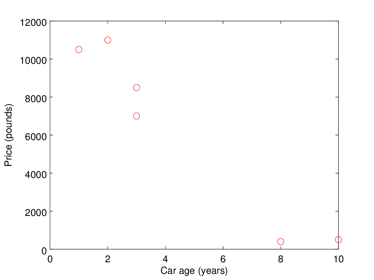
We could imagine a straight line drawn through the points on this graph. It's not (in this case) going to go exactly through every point, but we could place the line so that it goes as close to all the points as possible.
To say this in another way, we want to make the distance from the line to each point as small as possible. This is most often done by minimising the square of the distance from the line to each point.
We can describe the straight line in terms of two variables:
- The point at which it crosses the y-axis i.e. the predicted price of a brand new car. This is the intercept.
- The slope of the line - i.e. for every year of age, how much does the price change.
This is the equation for our line:
carPrice = slope * carAge + intercept
How can we find the best values for the intercept and the slope? Let's look at two different ways to do this.
An iterative approach
One approach is to start with some arbitrary values for the intercept and the slope. We work out what small changes we make to these values to move our line closer to the data points. Then we repeat this multiple times. Eventually our line will approach the optimum position.
First let's set up our data structures. We will use two Swift arrays for the car age and the car price:
let carAge: [Double] = [10, 8, 3, 3, 2, 1]
let carPrice: [Double] = [500, 400, 7000, 8500, 11000, 10500]
This is how we can represent our straight line:
var intercept = 0.0
var slope = 0.0
func predictedCarPrice(_ carAge: Double) -> Double {
    return intercept + slope * carAge
}
Now for the code which will perform the iterations:
let numberOfCarAdvertsWeSaw = carPrice.count
let numberOfIterations = 100
let alpha = 0.0001

for n in 1...numberOfIterations {
    for i in 0..<numberOfCarAdvertsWeSaw {
        let difference = carPrice[i] - predictedCarPrice(carAge[i])
        intercept += alpha * difference
        slope += alpha * difference * carAge[i]
    }
}
alpha is a factor that determines how much closer we move to the correct solution with each iteration. If this factor is too large then our program will not converge on the correct solution.
The program loops through each data point (each car age and car price). For each data point it adjusts the intercept and the slope to bring them closer to the correct values. The equations used in the code to adjust the intercept and the slope are based on moving in the direction of the maximal reduction of these variables. This is a gradient descent.
We want to minimise the square of the distance between the line and the points. We define a function J which represents this distance - for simplicity we consider only one point here. This function J is proportional to ((slope.carAge + intercept) - carPrice)) ^ 2.
In order to move in the direction of maximal reduction, we take the partial derivative of this function with respect to the slope, and similarly for the intercept. We multiply these derivatives by our factor alpha and then use them to adjust the values of slope and intercept on each iteration.
Looking at the code, it intuitively makes sense - the larger the difference between the current predicted car Price and the actual car price, and the larger the value of alpha, the greater the adjustments to the intercept and the slope.
It can take a lot of iterations to approach the ideal values. Let's look at how the intercept and slope change as we increase the number of iterations:
| Iterations | Intercept | Slope | Predicted value of a 4 year old car |
|---|---|---|---|
| 0 | 0 | 0 | 0 |
| 2000 | 4112 | -113 | 3659 |
| 6000 | 8564 | -764 | 5507 |
| 10000 | 10517 | -1049 | 6318 |
| 14000 | 11374 | -1175 | 6673 |
| 18000 | 11750 | -1230 | 6829 |
Here is the same data shown as a graph. Each of the blue lines on the graph represents a row in the table above.
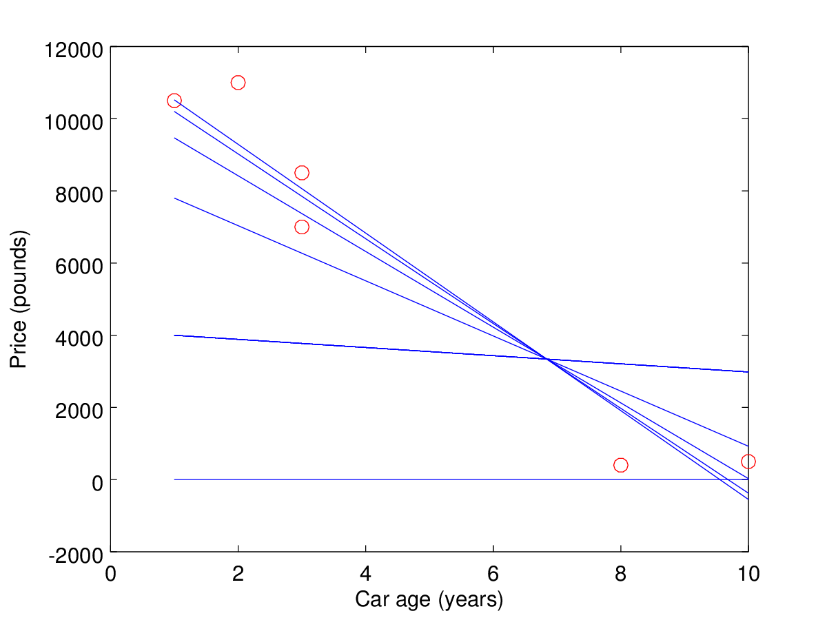
After 18,000 iterations it looks as if the line is getting closer to what we would expect (just by looking) to be the correct line of best fit. Also, each additional 2,000 iterations has less and less effect on the final result - the values of the intercept and the slope are converging on the correct values.
A closed form solution
There is another way we can calculate the line of best fit, without having to do multiple iterations. We can solve the equations describing the least squares minimisation and just work out the intercept and slope directly.
First we need some helper functions. This one calculates the average (the mean) of an array of Doubles:
func average(_ input: [Double]) -> Double {
    return input.reduce(0, +) / Double(input.count)
}
We are using the reduce Swift function to sum up all the elements of the array, and then divide that by the number of elements. This gives us the mean value.
We also need to be able to multiply each element in an array by the corresponding element in another array, to create a new array. Here is a function which will do this:
func multiply(_ a: [Double], _ b: [Double]) -> [Double] {
    return zip(a,b).map(*)
}
We are using the map function to multiply each element.
Finally, the function which fits the line to the data:
func linearRegression(_ xs: [Double], _ ys: [Double]) -> (Double) -> Double {
    let sum1 = average(multiply(ys, xs)) - average(xs) * average(ys)
    let sum2 = average(multiply(xs, xs)) - pow(average(xs), 2)
    let slope = sum1 / sum2
    let intercept = average(ys) - slope * average(xs)
    return { x in intercept + slope * x }
}
This function takes as arguments two arrays of Doubles, and returns a function which is the line of best fit. The formulas to calculate the slope and the intercept can be derived from our definition of the function J. Let's see how the output from this line fits our data:
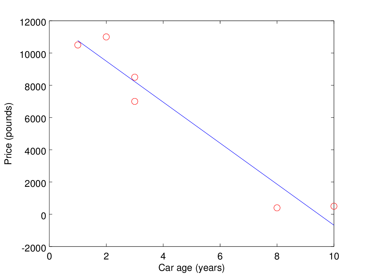
Using this line, we would predict a price for our 4 year old car of £6952.
Summary
We've seen two different ways to implement a simple linear regression in Swift. An obvious question is: why bother with the iterative approach at all?
Well, the line we've found doesn't fit the data perfectly. For one thing, the graph includes some negative values at high car ages! Possibly we would have to pay someone to tow away a very old car... but really these negative values just show that we have not modelled the real life situation very accurately. The relationship between the car age and the car price is not linear but instead is some other function. We also know that a car's price is not just related to its age but also other factors such as the make, model and engine size of the car. We would need to use additional variables to describe these other factors.
It turns out that in some of these more complicated models, the iterative approach is the only viable or efficient approach. This can also occur when the arrays of data are very large and may be sparsely populated with data values.
Written for Swift Algorithm Club by James Harrop