All-Pairs Shortest Paths
The All-Pairs shortest path problem simultaneously computes the shortest path from each node in the graph to each other node, provided a path exists for each pair. In the naive approach, we could simply compute a single-source shortest path from each node to each other node. The number of shortest paths computed is then bound by O(V^2), where V is the number of vertices in the graph. Because SSSP is also bounded by O(V^2), the total running time for the naive approach would be O(V^4).
However, by applying a dynamic approach on the adjacency matrix of the graph, a running time of O(V^3) is achievable, using the Floyd-Warshall algorithm. Floyd-Warshall iterates through an adjacency matrix, and for each pair of start(i) and end(j) vertices it considers if the current distance between them is greater than a path taken through another vertex(k) in the graph (if paths i ~> k and k ~> j exist). It moves through an adjacency matrix for every vertex k applying its comparison for each pair (i, j), so for each k a new adjacency matrix D(k) is derived, where each value d(k)[i][j] is defined as:

where w[i][j] is the weight of the edge connecting vertex i to vertex j in the graph's original adjacency matrix.
When the algorithm memoizes each refined adjacency and predecessor matrix, its space complexity is O(V^3), which can be optimised to O(V^2) by only memoizing the latest refinements. Reconstructing paths is a recursive procedure which requires O(V) time and O(V^2) space.
Example
For the following weighted directed graph
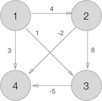
the adjacency matrix representation w is

Calculating shortest paths' weights
At the beginning of the algorithm, D(0) is the same as w, with the following exceptions to accommodate the comparison function:
- vertices with no path connecting them have the
øreplaced with∞ - the diagonal has all
0s
Here are all the adjacency matrices derived when perform Floyd-Warshall on the above graph:


with the last being the result, which tells for each pair of starting and ending vertices, the total weight of the shortest path connecting them. During the step where k = 2, the comparison that winds up changing the top right value from 2 to -4 goes like this:
k = 2, i = 0, j = 3
d(k-1)[i][j] => d(1)[0][3] = 2
d(k-1)[i][k] => d(1)[0][2] = 1
d(k-1)[j][k] => d(1)[2][3] = -5
therefore min(2, 2 + -5) => min(2, -4) produces a new weight of -4 for the element at d(2)[0][3], meaning that the shortest known path 1 ~> 4 before this step was from 1 -> 2 -> 4 with a total weight of -2, and afterwards we discovered a shorter path from 1 -> 3 -> 4 with a total weight of -4.
Reconstructing shortest paths
This algorithm finds only the lengths of the shortest paths between all pairs of nodes; a separate bookkeeping structure must be maintained to track predecessors' indices and reconstruct the shortest paths afterwards. The predecessor matrices at each step for the above graph follow:


Project Structure
The provided xcworkspace allows working in the playground, which imports the APSP framework target from the xcodeproj. Build the framework target and rerun the playground to get started. There is also a test target in the xcodeproj.
In the framework:
- protocols for All-Pairs Shortest Paths algorithms and results structures
- an implementation of the Floyd-Warshall algorithm
TODO
- Implement naive
O(V^4)method for comparison - Implement Johnson's algorithm for sparse graphs
- Implement other cool optimized versions
References
Chapter 25 of Introduction to Algorithms, Third Edition by Cormen, Leiserson, Rivest and Stein https://mitpress.mit.edu/books/introduction-algorithms
Written for Swift Algorithm Club by Andrew McKnight